Deep learning for Hidden Markov model
In this project, we study how we can use deep learning techniques in Hidden Markov model for analyzing time-series data.
References:
- Paper: Krishnan, Rahul, Uri Shalit, and David Sontag. “Structured inference networks for nonlinear state space models.” In Proceedings of the AAAI conference on artificial intelligence, vol. 31, no. 1. 2017.
- Code: deepHMM
Application example - A drug treatment study where we have data in cell-line x time x cnv format, for example 20 x 160 x 88 where 88 is pseudobulk CNV profile from cells in 160 time-points treated with a drug in 20 different cell lines. Our interest is to understand how CNV profile changes i.e. given a profile at time $t$ we want to predict changes at time $t+1$.
Hidden Markov process: Single vs Multi Time-Point Generative Assumptions
In the case of single time-point data, we assume that the observed data matrix cells x genes/cnv (for example, 20 x 88) is generated from a set of low-dimensional latent variables cells x factors (e.g., 20 x 10). In this setting, each cell’s observed profile is generated from its underlying 10 latent factors.
In the case of multiple time-point data, the observed data now has the form cells x time x genes/cnv (for example, 20 x 160 x 88). We continue to assume that each time-point’s data is generated from the same set of 10 latent factors i.e. at each time $ t $, the observed data is generated from 10 latent factors. However, since this is time-series data, we must model how these factors evolve over time i.e. how the latent variables change from $ t-1 $ to $ t $.
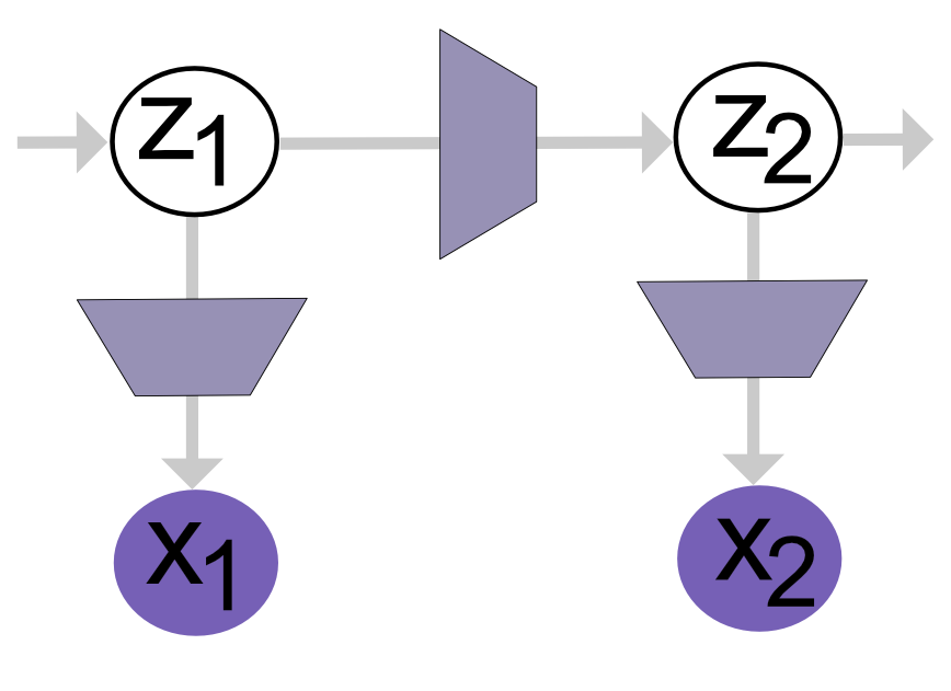
To do this, we introduce a Markov process: we assume that the latent state at time $ t $ depends only on the latent state at time $ t-1 $ (first-order Markov property).
To fully specify this generative process for time-series data, we need the following components:
-
Prior: Given $ z_{t-1} $, what is the probability distribution of $ z_t $? This models how the latent state evolves over time.
-
Posterior: Given $ z_{t-1} $ and the observed data at time $ t $, what is the updated distribution for $ z_t $? This is used during training to perform inference.
-
Emission: Given the latent state $ z_t $, how is the observed data at time $ t $ generated?
Variational Hidden Markov model:
Our aim here is to learn the generative process for time-series data using a Variational Hidden Markov Model (VHMM).
- Transition model: How latent state transit from one time step to next. The prior $z_t$ is updated as $p(z_t | z_{t-1})$ transition logits [z_dim x z_dim]
self.transition_logits = nn.Parameter(torch.randn(z_dim, z_dim))
- Variational posterior: We use variational inference to approximate posterior distribution. The posterior $z_t$ is updated as Variational $q(z_t | x_1:T)$ - approximate posterior.
self.q_logits = nn.Parameter(torch.randn(1, z_dim))
- Emission model: The model generates observed data at $t$. The new data at $t$ is generated from $z_t$ posterior. The $p(x_t | z_t)$s: emission parameters [z_dim x input_dim], assume Bernoulli
self.emission_logits = nn.Parameter(torch.randn(z_dim, input_dim))
Simple to Deep HMM
In a Simple VHMM, the latent state $ z_t $ is a discrete variable (with dimension $ z_{\text{dim}} $), and both the transition and emission models are parameterized by fixed matrices. The entire temporal structure of the model depends on a fixed transition matrix and emission matrix.
In a Deep HMM (DHMM), we add the following deep components:
-
The latent variable $ z_t $ is now continuous, typically modeled as a Gaussian:
-
The transition model is parameterized by a neural network to allow flexible and nonlinear transitions across time.
- The variational posterior is also parameterized by a neural network:
where $ h_t $ is an RNN hidden state summarizing the data.
- The emission model is parameterized by a neural network (MLP), allowing a flexible mapping from continuous latent to the observed space.
Deep HMM model
The Deep HMM consists of the following modules:
-
RNN Encoder: encodes each time point feature vector into a high-dimensional embedding $ h $.
(Example: 88 features to 600-dimensional embedding) -
Transition Network: computes the prior distribution $ p(z_t | z_{t-1}) $
-
Post-transition Network: computes the approximate posterior $ q(z_t | z_{t-1}, x_{t:T}) $
-
Emitter Network: models the likelihood $ p(x_t | z_t) $
RNN Encoder
The encoder architecture:
(rnn): Encoder(
  (rnn): GRU(88, 600, batch_first=True)
)
- Input dimension: 88
- RNN hidden dimension: 600
Example input shape:
inputs.shape # torch.Size([20, 160, 88])
In this example:
- Batch size = 20 (20 cell lines)
- 160 time points per cell line
- 88 feature measurements per time point
We aim to encode this data from 88D to 600D embeddings.
Since not all conditions have all time points, we provide a length vector to tell RNN which time points are present for each sample.
For example, a batch might have max 96 time points, not 160, so the RNN only trains up to t=96. So,for training this batch we dont need to update parameters for 97 and above time points. pyTorch RNN (GRU) module has padding function to take care of this as long as we provide what time points data we have for each condition.
We also provide an initial hidden state $ h_0 $:
self.h_0 = nn.Parameter(torch.zeros(1, 1, self.rnn_dim))
# torch.Size([1, 1, 600])

h_0 = self.h_0.expand(1, batch_size, self.rnn.hidden_size).contiguous()
# torch.Size([1, 20, 600])
Running the RNN encoder:
_, rnn_out = self.rnn(x_rev, x_lens, h_0)

rnn_out.shape
# torch.Size([20, 96, 600])
So, inputs of shape [20, 160, 88] are encoded to embeddings [20, 96, 600]. But the RNN model will have parameters for the entire dataset.
RNN parameter sizes:
for name, param in self.rnn.named_parameters():
    print(f"{name}: {param.shape}")
| Parameter | Shape | Description |
|---|---|---|
| weight_ih_l0 | [1800, 88] | input → hidden (for 3 gates) |
| weight_hh_l0 | [1800, 600] | hidden → hidden (for 3 gates) |
| bias_ih_l0 | [1800] | |
| bias_hh_l0 | [1800] |
Why 1800? Because GRU has 3 gates:
| Gate | Size |
|---|---|
| Update gate (z) | 600 |
| Reset gate (r) | 600 |
| New gate (n) | 600 |
| Total | 1800 |
Transition Network
For each time point $ t $, we estimate prior $ z_t $:
z_prior, z_prior_mu, z_prior_logvar = self.trans(z_prev)
Architecture:
(trans): GatedTransition(
  (gate): Sequential(
    (0): Linear(100 → 200)
    (1): ReLU
    (2): Linear(200 → 100)
    (3): Sigmoid
  )
  (proposed_mean): Sequential(
    (0): Linear(100 → 200)
    (1): ReLU
    (2): Linear(200 → 100)
  )
  (z_to_mu): Linear(100 → 100)
  (z_to_logvar): Linear(100 → 100)
)
Interpretation:
Given $ z_{t-1} $, output $p(z_t | z_{t-1})$ as Gaussian parameters $ (\mu, \log \sigma^2) $.
self.trans is transition network to calculate z_t prior i.e. Given the latent z_{t-1} corresponding to the time step t-1 we return the mean and scale vectors that parameterize the (diagonal) gaussian distribution p(z_t | z_{t-1}).
Postnet Network
Posterior update:
z_t, z_mu, z_logvar = self.postnet(z_prev, rnn_out[:,t,:])
Architecture:
(postnet): PostNet(
  (z_to_h): Sequential(
    (0): Linear(100 → 600)
    (1): Tanh
  )
  (h_to_mu): Linear(600 → 100)
  (h_to_logvar): Linear(600 → 100)
)
Interpretation:
Parameterizes $ q(z_t | z_{t-1}, x_{t:T}) $, where $ x_{t:T} $ is encoded via RNN $ h_t $.
self.postnet gives posterior distribution of latent variable conditioned on input sequence (for training) i.e. Parameterizes q(z_t|z_{t-1}, x_{t:T}), which is the basic building block of the inference (i.e. the variational distribution). The dependence on x_{t:T} is through the hidden state of the RNN.
Emitter Network
| Finally, given posterior $ z_t $, model $ p(x_t | z_t) $: |
logit_x_t = self.emitter(z_t).contiguous()
Architecture:
(emitter): Sequential(
  (0): Linear(100 → 100)
  (1): ReLU
  (2): Linear(100 → 100)
  (3): ReLU
  (4): Linear(100 → 88)
  (5): Sigmoid
)
Interpretation:
Maps $ z_t $ to Bernoulli likelihood for observed features (88-dimensional).
Once we have posterior distribution z_t, we calculate model likelihood i.e. Parameterizes the bernoulli observation likelihood p(x_t|z_t). The emitter network is just a sequential network to map latent dim to feature dim with sigmoid function.
Loss Calculation
- KL divergence:
kl_div(z_mu, z_logvar, z_prior_mu, z_prior_logvar)
- Reconstruction loss (Bernoulli):
nn.BCEWithLogitsLoss(logit_x_t, x[:,t,:])
Conclusion
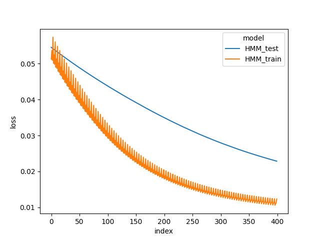
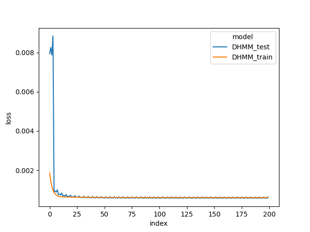
We use simulated data as described in deepHMM tutorial. The set consists of 200 cell lines, each with 160 time points and 88 features.
When we compare the loss trace during model training in the below figures, DeepHMM train and test loss are lower than HMM train loss. The results show that the DeepHMM is more expressive model due to RNN and neural network modules, and captures a higher resolution of temporal dependencies in the data.
The code used in the analyses are available deepHMM.

