Evaluate scNET model to integrate protein interaction network with single-cell expression data
In this project, we study the scNET paper and understand how the model utilizes prior biological knowledge database, such as protein-protein interaction network, to improve the latent space representation of single-cell data.
The authors in the paper present an interesting approach to fuse the dual latent space, one derived from a known protein-protein interaction network and the other from single-cell gene expression data. The authors highlight that incorporating protein interaction data into the model enhances gene annotation, identifies gene-gene relationships, and facilitates pathway analysis across diverse cell types and biological conditions.
-
scNET Github repo
First, let us download and explore the example data.
import gdown
import scanpy as sc

download_url = f'https://drive.google.com/uc?id=1C_G14cWk95FaDXuXoRw-caY29DlR9CPi'
output_path = './data/example.h5ad'
gdown.download(download_url, output_path, quiet=False)

### scfuse is a local wrapper object for the original scNET model described in the paper
import scfuse

import pandas as pd
import scanpy as sc

adata = sc.read_h5ad("./data/example.h5ad")

ppi_net = pd.read_csv("./resources/format_h_sapiens.csv")[["g1_symbol","g2_symbol","conn"]].drop_duplicates()
Here, for single-cell data, the anndata object contains gene expression data, cell x gene consisting of 9172 cells and ~18,000 genes.
For protein-protein interaction network data, ppi_net dataframe has three columns gene1, gene2, and conn score. The dataframe has ~500k edges with connection values from 0.1 to 1.0
We build a gene-gene network from the provided interaction database. We only analyze highly variable genes.
adata = adata[:,adata.var.highly_variable]
net, ppi, node_feature = scfuse.model.scnet.build_network(adata, ppi_net)
We have:
-
net is filtered dataframe such that now conn has only 2598 edges from ~500k with scores from 0.5 to 1.0.
-
ppi is a networkx graph object where edges are 2598 gene-gene edges and nodes are 1359 genes (out of 3023 highly variable genes present in the original ppi network)
-
node_feature is a gene x cell dataframe where we have 1359 genes and 9172 cells.
so we have–
- adata is anndata with 9172 cells and 3023 highly variable genes
- net is dataframe with 2598 rows of gene-gene edge score
- ppi is graph of 1359 genes and 2598 edges
- node_feature is single-cell gene expression count dataframe with 1359 genes and 9172 cells
Next, we construct cell-cell similarity graph using connectivity scores in the original anndata.
import networkx as nx
import numpy as np
import torch
from torch_geometric.utils import  convert

adata = adata[:,node_feature.index]
### now have same genes in both graph and anndata

## cell-cell network
cell_graph = adata.obsp["distances"].toarray()
cell_graph = (cell_graph > 0).astype(int)
cell_graph = nx.from_numpy_array(np.matrix(cell_graph))
cci_geo = convert.from_networkx(cell_graph)
knn_edge_index = cci_geo.edge_index

## protein-protein network
ppi_edge_index, _ = scfuse.model.scnet.nx_to_pyg_edge_index(ppi)

## count data in tensor
row_x = node_feature.T.values
row_x_label = np.array(range(node_feature.shape[1]))
row_x = torch.tensor(row_x, dtype=torch.float32).cpu()
Here, knn_edge_index is cell-cell similarity graph edges for 9172 cells.
Recap of our data variables:
- single cell gene count dataframe
- node_feature.shape -> gene x cell (1359, 9172)
- count data converted to tensor
- row_x.shape -> torch.Size([9172, 1359])
- row_x_label.shape -> (9172,)
- gene-gene network for 1359 genes
- ppi_edge_index.shape -> gene-gene edges torch.Size([2, 5196])
- ppi_edge_index[0,:].max() -> tensor(1358)
- cell-cell network for 9172 cells
- knn_edge_index.shape -> cell-cell edges torch.Size([2, 374704])
- knn_edge_index[0,:].max() -> tensor(9171)
Important: Training strategy
- Use cell-cell network as dataloader to get batch of cells (dynamic)
- Load expression data and protein-protein network on GPU (static)
from torch.utils.data import DataLoader
from torch_geometric.data import Data

device ='cuda'
data = Data(row_x,ppi_edge_index)
data = data.to(device)

knn_dataset = scfuse.dataloader_graph.KNNDataset(knn_edge_index)
batch_size = 100
knn_loader = DataLoader(knn_dataset,batch_size=batch_size, shuffle=True, drop_last=False)
Model setup
INTER_DIM = 250
EMBEDDING_DIM = 75
NUM_LAYERS = 3

model = scfuse.model.scnet.scNET( data.x.shape[1],batch_size *2,
INTER_DIM, EMBEDDING_DIM, INTER_DIM, EMBEDDING_DIM, lambda_rows = 1, lambda_cols=1,num_layers=NUM_LAYERS).to(device)

scNET(
 (encoder): MutualEncoder(
 (rows_layers): ModuleList(
 (0-2): 3 x Sequential(
 (0) - SAGEConv(200, 200, aggr=mean): x, edge_index -> x1
 (1) - Dropout(p=0.25, inplace=False): x1 -> x2
 (2) - LeakyReLU(negative_slope=0.01, inplace=True): x2 -> x2
 )
 )
 (cols_layers): ModuleList(
 (0-2): 3 x Sequential(
 (0) - SAGEConv(1359, 1359, aggr=mean): x, edge_index -> x1
 (1) - LeakyReLU(negative_slope=0.01, inplace=True): x1 -> x1
 (2) - Dropout(p=0.25, inplace=False): x1 -> x2
 )
 )
 )
 (rows_encoder): DimEncoder(
 (encoder): Sequential(
 (0) - GCNConv(200, 250): x, edge_index -> x1
 (1) - LeakyReLU(negative_slope=0.01, inplace=True): x1 -> x1
 (2) - Dropout(p=0.25, inplace=False): x1 -> x2
 )
 (atten_layer): TransformerConv(250, 75, heads=1)
 )
 (cols_encoder): DimEncoder(
 (encoder): Sequential(
 (0) - GCNConv(1359, 250): x, edge_index -> x1
 (1) - LeakyReLU(negative_slope=0.01, inplace=True): x1 -> x1
 (2) - Dropout(p=0.25, inplace=False): x1 -> x2
 )
 (atten_layer): TransformerConvReducrLayer(250, 75, heads=1)
 )
 (feature_decodr): FeatureDecoder(
 (decoder): Sequential(
 (0): Linear(in_features=75, out_features=250, bias=True)
 (1): Dropout(p=0, inplace=False)
 (2): ReLU()
 (3): Linear(in_features=250, out_features=250, bias=True)
 (4): Dropout(p=0, inplace=False)
 (5): ReLU()
 (6): Linear(in_features=250, out_features=1359, bias=True)
 (7): Dropout(p=0, inplace=False)
 )
 )
 (ipd): InnerProductDecoder()
 (feature_critarion): MSELoss()
)
Model training
EPS = 1e-15
batch_size = 100
device = 'cuda'
max_epoch = 100

def update_batch(batch, c_x_indx_map):
    for i in range(batch.size(0)):
    for j in range(batch.size(1)):
    if batch[i, j].item() in c_x_indx_map:
    batch[i, j] = c_x_indx_map[batch[i, j].item()]
    return batch

optimizer = torch.optim.Adam(model.parameters(), lr=0.0001, weight_decay=1e-5)

for epoch in range(max_epoch):

    total_row_loss = 0
    total_col_loss = 0

    for _,batch in enumerate(knn_loader):

    ## get cell indexes
    c_x_indxs =  batch.flatten().unique()

    if len(c_x_indxs) != batch_size *2:
    continue

    ## expression data
    c_x = data.x[c_x_indxs,:].clone()
    c_x = c_x.T

    c_x_indx_map = {int(y):x for x,y in enumerate(c_x_indxs)}

    updated_batch = update_batch(batch, c_x_indx_map)

    row_embed, col_embed, out_features = model(c_x.to(device), updated_batch.T.to(device), data.edge_index)


    row_loss = model.recon_loss(row_embed, data.edge_index,sig=True)


    out_features = (out_features - (out_features.mean(axis=0)))/ (out_features.std(axis=0)+ EPS)
    reg = model.recon_loss(out_features.T, data.edge_index, sig=False)
    col_loss = model.feature_critarion(c_x.T, out_features)

    loss =  row_loss + col_loss + reg
    optimizer.zero_grad()
    loss.backward()
    optimizer.step()

    total_row_loss += row_loss.detach().cpu().numpy()
    total_col_loss += (col_loss.detach().cpu().numpy()+reg.detach().cpu().numpy())

    print('epoch '+ str(epoch)+ '  rl...'+ str(total_row_loss) + '  cl...'+ str(total_col_loss))


torch.save(model.state_dict(),'results/scfuse_example_model.pt')
Inference
model.load_state_dict(torch.load('results/scfuse_example_model.pt', weights_only=True, map_location=torch.device(device)))

model.eval()

dfl = pd.DataFrame()
for _,batch in enumerate(knn_loader):

    c_x_indxs =  batch.flatten()
    c_x = data.x[c_x_indxs,:].clone()
    c_x = c_x.T

    if c_x.shape[1] != batch_size * 2:
    continue

    c_x_indx_map = {int(y):x for x,y in enumerate(c_x_indxs)}

    c_x_indxs_before = c_x_indxs.detach().cpu().numpy().copy()
    updated_batch = update_batch(batch, c_x_indx_map)

    row_embed, col_embed, out_features = model(c_x.to(device), updated_batch.T.to(device), data.edge_index)

    df = pd.DataFrame(col_embed.detach().cpu().numpy())
    df.index = c_x_indxs_before

    dfl = pd.concat([dfl, df[~df.index.isin(dfl.index)]])

dfl = dfl[~dfl.index.duplicated(keep='last')]
dfl = dfl.sort_index()

dfl.to_parquet('results/scfuse_embed.pt',compression='gzip')
Validation
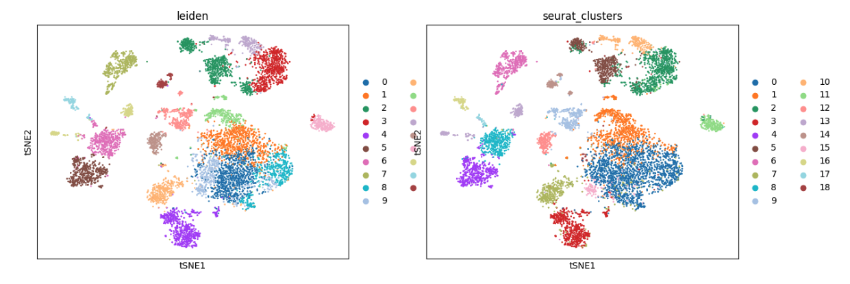
We compare Leiden labels from new latent spaces generated in this analysis with the original Seurat cluster labels.
dfl = pd.read_parquet('results/scfuse_embed.pt')
dfl.index = adata.obs.index.values
adata.obsm['scfuse'] = dfl
adata.obs.leiden = None

import matplotlib.pylab as plt

sc.pp.neighbors(adata,use_rep='scfuse')
sc.tl.tsne(adata)
sc.tl.leiden(adata)
sc.pl.tsne(adata,color=['leiden','seurat_clusters'])
plt.tight_layout()
plt.savefig('results/scfuse_umap_example.png')

Conclusion
scNET offers a novel approach to integrating protein interaction network data with single-cell gene expression data. The model training technique, which involves three data variables—expression data, cell-cell graph, and gene-gene graph—is a critical step in learning the scNET model. It teaches us how to batch cells using a cell-cell graph. However, this approach may not be scalable as we have to store expression and protein network data on GPU. It will be interesting to update the model so that we can batch the entire data triplet (expression data along cell and graph networks) for scalability.
The project code used to evaluate scNET model is available scNET_eval.