Multimodal analysis for discovery of complex trait genetics
In this project, I am interested in exploring the integration of multimodal (scATAC + scRNA + SNPs) data to reveal novel disease mechanisms.
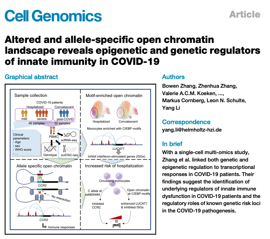
I will use data from Zhang et al 2023 paper. The paper analyzes data from COVID-19 patients and examines the connections between genetic variations, epigenetic factors, and immune responses at the cellular level.
I will extend the original analyses to approximate cell-type-resolved chromatin accessibility (caQTL) profiles. This approach will link genetic, epigenetic, and transcriptional data to identify regulatory mechanisms in patients with COVID-19.
scRNAseq analysis
library(Seurat)
library(ArchR)
library(ggplot2)

sc_data <- readRDS("data/Monocytes_scRNAseq.rds")
sc_data <- UpdateSeuratObject(sc_data)

colnames(sc_data@meta.data)
unique(sc_data@meta.data$celltype.idL0)
pdf("UMAP_scRNA.pdf",height=4,width=8)
p1 <- DimPlot(sc_data,label=T,group.by = "celltype.idL0")
p2 <- DimPlot(sc_data,label=T,group.by = "Severity")
p <- p1 + p2
plot(p)
dev.off()
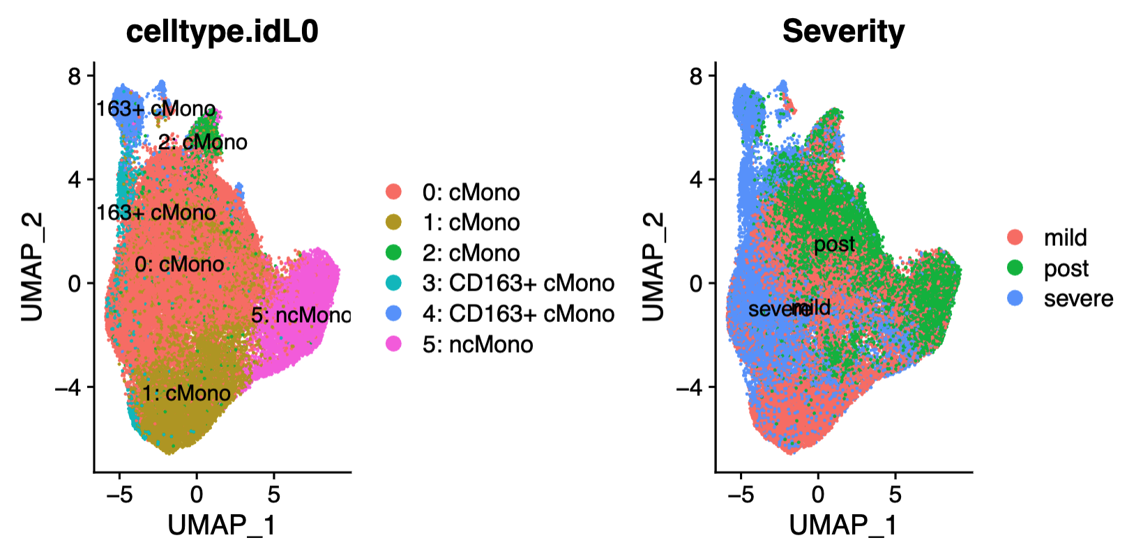
The scRNAseq data consists of 25901 genes/features across 56569 cells within one assay. A total of 1,000 variable features were used for the analysis. Harmony was employed for data integration across COVID-19 patients.
scATACseq analysis
proj <- readRDS("data/Monocyte_scATACseq/Save-ArchR-Project.rds")

colnames(getCellColData(proj))

umapEmbedding <- getEmbedding(proj, embedding = "UMAP")
cellColData <- getCellColData(proj)

umapData <- data.frame(
  Cell = rownames(umapEmbedding),
  UMAP_1 = umapEmbedding[, 1],
  UMAP_2 = umapEmbedding[, 2],
  Clusters = cellColData[rownames(umapEmbedding), "Clusters"],
  predictedGroup = cellColData[rownames(umapEmbedding), "predictedGroup"],
  Severity = cellColData[rownames(umapEmbedding), "Severity"]
)

pdf("UMAP_scATAC.pdf",height=4,width=8)

p1 <- ggplot(umapData, aes(x = UMAP_1, y = UMAP_2, color = predictedGroup)) +
  geom_point(size = 0.5) +
  theme_minimal() +
  labs(title = "UMAP Colored by Clusters", x = "UMAP 1", y = "UMAP 2")

p2 <- ggplot(umapData, aes(x = UMAP_1, y = UMAP_2, color = Severity)) +
  geom_point(size = 0.5) +
  theme_minimal() +
  labs(title = "UMAP Colored by Clusters", x = "UMAP 1", y = "UMAP 2")

p <- p1 + p2
plot(p)
dev.off()
The ATACseq dataset comprises 24,919 genes/features and 10,596 single cells that passed basic quality control in the arrow files. TSS enrichment measures the degree to which the transcription start site (TSS) is more accessible compared to its flanking regions. A score>10 is considered good accessibility. The dataset score is 13.9. The median number of unique fragments per cell is 5,389.5, indicating high-quality data. Also, doublet has been calculated and filtered.
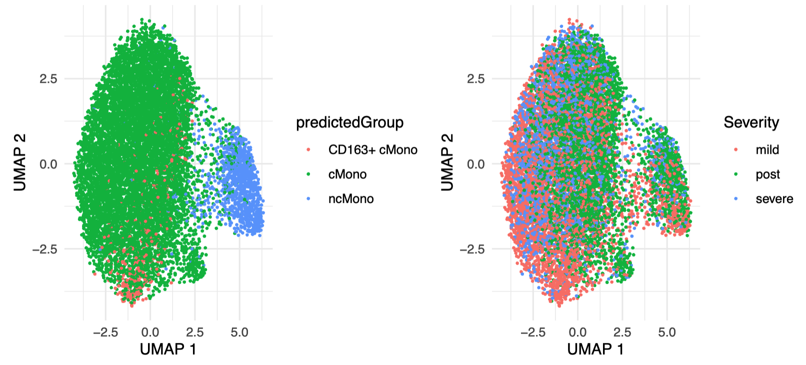
Integration was conducted using addGeneIntegrationMatrix function in archR. Briefly, both RNAseq and ATACseq chromatin accessiblility data (peaks) are projected onto low-dimensional latent space ( LSI for ATACseq and PCA for RNAseq). Cell matching across datasets based on similarity in this shared space, followed by gene expression imputation and cell type label transfer.
projDm <- addGeneIntegrationMatrix(
     ArchRProj = projDm,
     useMatrix = "GeneScoreMatrix",
     matrixName = "GeneIntegrationMatrix",
     reducedDims = "IterativeLSI",
     seRNA = scRNA,
     addToArrow = FALSE,
     groupRNA = "celltypeL0",
     nameCell = "predictedCell_Un",
     nameGroup = "predictedGroup_Un",
     nameScore = "predictedScore_Un"
)
Now, let’s outline the analysis plan:
Step 1: Use scATACseq analysis to extract the gene score matrix, which provides gene x cell chromatin accessibility data.
Step 2: Create pseudobulk data based on cell types for each patient. We transfer cell-type labels from single-cell data integration analysis. Here, we generate gene x celltype_patient pseudobulk data.
Step 3: Use publicly available COVID-19 GWAS summary statistics and select significantly disease-associated variants.
Step 4: Obtain patient-level genotype data.
Once we generate three main data inputs:
- Pseudobulk chromatin accessibility data for each cell type and patient
- Significantly COVID-19-associated variants data
- Patient-level genotype data
Next, we focus on our main data analysis question:
Cell-type specific gene - chromatin accessibility association
Now, lets follow the analysis plan:
Step 1: Use scATACseq analysis to extract the gene score matrix, which provides gene x cell chromatin accessibility data.
proj <- readRDS("data/Monocyte_scATACseq/Save-ArchR-Project.rds")

# Update Arrow file paths
oldArrowPaths <- getArrowFiles(proj)
newArrowPaths <- gsub(
  "/vol/projects/BIIM/Covid_50MHH/scATAC/analysis_new2/projMono_uniq/",
  "/data/sishir/projects/qtl_wrksh/data/Monocyte_scATACseq/",
  oldArrowPaths,
  fixed = TRUE
)
names(newArrowPaths) <- names(oldArrowPaths)
newSampleColData <- DataFrame(
  ArrowFiles = newArrowPaths[rownames(proj@sampleColData)],
  row.names = rownames(proj@sampleColData)
)
proj@sampleColData <- newSampleColData
getArrowFiles(proj)


# Extract GeneScoreMatrix
geneScoreMat <- getMatrixFromProject(
  ArchRProj = proj,
  useMatrix = "GeneScoreMatrix"
)
counts <- assay(geneScoreMat)
rownames(counts) <- rowData(geneScoreMat)$name
Here, counts matrix is a cell-by-gene matrix containing gene activity scores, not peak counts or direct gene expression. These scores are inferred from chromatin accessibility (e.g., promoter and enhancer regions) in scATAC-seq data, serving as a proxy for gene expression before scRNA-seq integration.
Rows are genes (24919), columns are cells (10596)
Step 2: Create pseudobulk data based on cell types for each patient. We transfer cell-type labels from single-cell data integration analysis. Here, we generate gene x celltype_patient pseudobulk data.
Here, we focus on three cell types - classical, non-classical monocytes, and CD163+ classical monocytes.
colnames(getCellColData(proj))

# Get cell type assignment from single cell integration analysis
celltypes <- getCellColData(proj)$predictedGroup
patients <- getCellColData(proj)$patient

# Create unique patient-cell type combinations
combinations <- paste0(patients, "_", celltypes)
unique_combinations <- unique(combinations)

# Aggregate counts by patient and cell type (pseudobulk)
pseudobulk <- do.call(cbind, lapply(unique_combinations, function(combo) {
  idx <- which(combinations == combo)
  if (length(idx) > 0) {
    Matrix::rowSums(counts[, idx, drop = FALSE])
  } else {
    Matrix::Matrix(0, nrow = nrow(counts), ncol = 1)
  }
}))
colnames(pseudobulk) <- unique_combinations

gz <- gzfile("data/pseudobulk.csv.gz", "w")
write.csv(pseudobulk, file = gz, row.names = TRUE, col.names = TRUE)
close(gz)
Step 3: Use publicly available COVID-19 GWAS summary statistics and select significantly disease-associated variants.
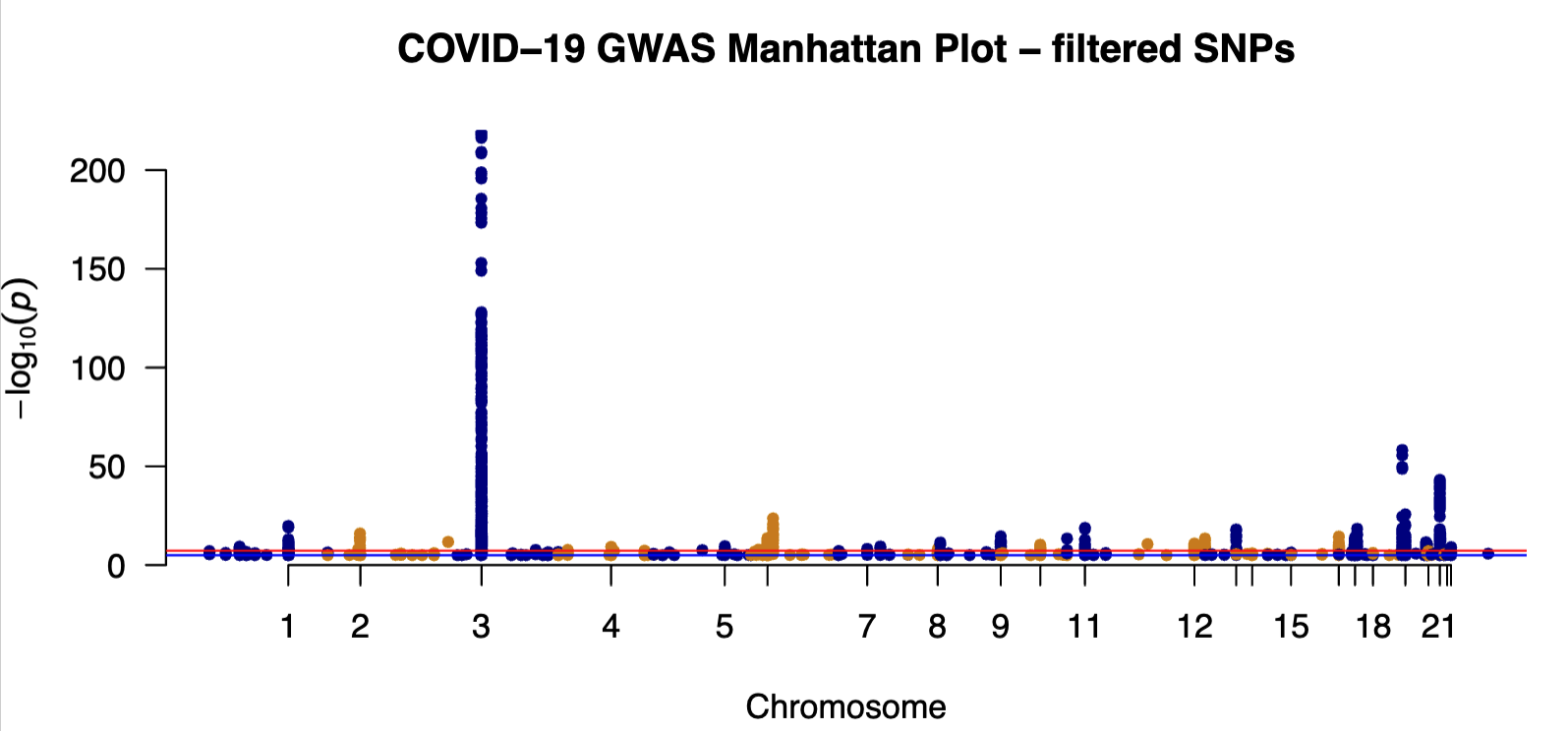
Here, we download COVID-19 GWAS summary statistics from COVID-19 host genetics initiative database. We use COVID19-hg GWAS meta-analyses round 7 for all population data.
The VCF file contains summary statistics for genetic variants, including columns like CHR, POS, REF, ALT, SNP, effect sizes (all_inv_var_meta_beta), standard errors (all_inv_var_meta_sebeta), p-values (all_inv_var_meta_p), allele frequencies (all_meta_AF), etc.
library(dplyr)
library(data.table)
library(qqman)

# Load GWAS data
gwas <- fread("data/summ_gwas.tsv")

# Rename columns if needed
colnames(gwas)[colnames(gwas) == "#CHR"] <- "CHR"
colnames(gwas)[colnames(gwas) == "POS"] <- "BP"
colnames(gwas)[colnames(gwas) == "all_inv_var_meta_p"] <- "P"

# Remove rows with NA or P=0
gwas <- gwas %>% filter(!is.na(P), P > 0)
gwas$SNP <- rownames(gwas)
gwas[, SNP := paste0("rs", SNP)]
gwas <- gwas[,c("SNP", "CHR", "BP", "P")]

pdf("GWAS_summary.pdf",height=4,width=8)
manhattan(gwas,
          chr = "CHR",
          bp = "BP",
          p = "P",
          snp = "SNP",
          col = c("blue4", "orange3"),
          genomewideline = -log10(5e-8),
          suggestiveline = -log10(1e-5),
          main = "COVID-19 GWAS Manhattan Plot - filtered SNPs")
dev.off()
Ok, now we have:
-
Summary GWAS data from COVID 19 patients where significant chr, position, and pvalues are estimated
-
Chromatin accessibility data from pseudobulk where gene accesibility score is aggregated by cell type and patient
-
We are missing donor level genotype data, we simulate the data as the original data has restricted access
library(data.table)

pseudobulk <- fread("data/pseudobulk.csv.gz")
rownames <- pseudobulk[[1]]
pseudobulk <- pseudobulk[, -1]
pseudobulk <- as.matrix(pseudobulk)
rownames(pseudobulk) <- rownames

# Normalize pseudobulk for a specific cell type
celltype <- "cMono"
cols <- grep(paste0("_", celltype, "$"), colnames(pseudobulk), value = TRUE)
pseudobulk_cmono <- pseudobulk[, cols]
pseudobulk_cmono <- t(scale(t(pseudobulk_cmono)))

celltype <- "ncMono"
cols <- grep(paste0("_", celltype, "$"), colnames(pseudobulk), value = TRUE)
pseudobulk_ncmono <- pseudobulk[, cols]
pseudobulk_ncmono <- t(scale(t(pseudobulk_ncmono)))


# Map significant SNPs to genes within 1Mb
gene_pos <- as.data.table(rowData(geneScoreMat))[, .(name, seqnames, start, end)]
setnames(gene_pos, c("gene", "chr", "start", "end"))
gene_pos[, `:=`(start_window = start - 1e6, end_window = end + 1e6)]

# Filter GWAS for significant SNPs
gwas_sig <- gwas[P < 5e-8, ]
gwas_sig[, CHR := as.character(CHR)] # Ensure CHR is character
gene_pos[, chr := as.character(chr)]
gwas_sig[, CHR := paste0("chr", CHR)]
gwas[, CHR := paste0("chr", CHR)]

# Join GWAS SNPs with genes
genes_overlapping <- gwas_sig[gene_pos,
                             .(SNP, gene, chr = CHR, pos = BP, P),
                             on = .(CHR == chr, BP >= start_window, BP <= end_window),
                             nomatch = 0]

genes_unique <- unique(genes_overlapping[, .(gene, chr)])
Association analysis: For each gene present in both summary GWAS data and ATACseq data, we estimate beta values for all the SNPs associated with the gene. Then we use cell-type specific chromatic accessibility for all donors and fit a linear model
-
chromatin_accessibilty_score ~ SNPs.
all_results <- list()

for ( gene in genes_unique$gene) {

  print(gene)

  # Get gene position
  gene_pos <- rowData(geneScoreMat)[rowData(geneScoreMat)$name == gene, ]
  chr <- as.character(gene_pos$seqnames)
  start <- gene_pos$start - 1e6
  end <- gene_pos$end + 1e6

  # Subset GWAS SNPs in gene region
  gwas_subset <- gwas[gwas$CHR == chr & gwas$BP >= start & gwas$BP <= end, ]

  # Estimate summary stats from pvalues
  gwas_subset[, beta := qnorm(P/2, lower.tail = FALSE) * sign(runif(.N, -1, 1))]
  gwas_subset[, se := abs(beta / qnorm(P/2, lower.tail = FALSE))]
  gwas_subset[, freq := 0.5] # Default MAF
  gwas_subset[, N := 1000] # Default sample size


  # now we have two vectors:
  #(1) beta vector from gwas_subset data calculated based on pvalues from summary statistics
  #(2) chromatin accesibility vector for gene in diffrent patients as pseudobulk_ct[gene,]

  ## simulate genotype using estimation from gwas summary
  n_donors_ncmono <- length(pseudobulk_ncmono[gene,])
  n_donors_cmono <- length(pseudobulk_cmono[gene,])
  n_donors <- max(n_donors_ncmono, n_donors_cmono)

  if (any(is.nan(pseudobulk_ncmono[gene, ]) | is.na(pseudobulk_ncmono[gene, ])) || any(is.nan(pseudobulk_cmono[gene, ]) | is.na(pseudobulk_cmono[gene, ]))) next

  geno <- matrix(NA, nrow = nrow(gwas_subset), ncol = n_donors)
  rownames(geno) <- gwas_subset$SNP
  for (i in 1:nrow(gwas_subset)) {
    maf <- gwas_subset$freq[i]
    # Simulate genotypes (0, 1, 2) under Hardy-Weinberg equilibrium
    geno[i, ] <- rbinom(n_donors, 2, maf)
  }
  geno <- t(geno)  # Donors x SNPs


# Fit linear model
fit_lm <- function(scores, geno, n_donors) {
  results <- lapply(1:ncol(geno), function(i) {
    snp <- colnames(geno)[i]
    valid_idx <- 1:min(n_donors, nrow(geno))  # Match donor count
    lm_fit <- lm(scores ~ geno[valid_idx, i])
    coef_summary <- summary(lm_fit)$coefficients
    if (nrow(coef_summary) > 1) {
      beta <- coef_summary[2, 1]
      se <- coef_summary[2, 2]
      pval <- coef_summary[2, 4]
    } else {
      beta <- NA
      se <- NA
      pval <- 1
    }
    list(beta = beta, se = se, pval = pval)
  })
  list(
    beta = sapply(results, function(x) x$beta),
    se = sapply(results, function(x) x$se),
    pval = sapply(results, function(x) x$pval)
  )
}

results_ncmono <- fit_lm(pseudobulk_ncmono[gene,], geno, n_donors_ncmono)
results_cmono <- fit_lm(pseudobulk_cmono[gene,], geno, n_donors_cmono)

gene_results <- data.table(
    gene = gene,
    SNP = rep(gwas_subset$SNP, 2),
    cell_type = rep(c("ncMono", "cMono"), each = nrow(gwas_subset)),
    beta = c(results_ncmono$beta, results_cmono$beta),
    se = c(results_ncmono$se, results_cmono$se),
    pvalue = c(results_ncmono$pval, results_cmono$pval),
    gwas_beta = rep(gwas_subset$beta, 2),
    chr = chr,
    pos = gwas_subset$BP
  )

all_results[[gene]] <- gene_results

}

results <- do.call(rbind, all_results)

# Step 4: Identify cell-type-specific associations
results[, sig := pvalue < 0.05]

results[, beta_diff := abs(beta - shift(beta, n = sum(cell_type == "ncMono"), type = "lead")), by = gene]
results[, cell_specific := sig & beta_diff > 0.1]  # Threshold for specificity
results <- results[sig == TRUE | cell_specific == TRUE]
write.csv(results, "data/snp_association_significant_genes_ncMono_cMono.csv")
Now, we select genes from the results in the original paper.
We compare whether our analyses identified the same genes as highly associated with disease variants.
library(data.table)
library(ggplot2)
results <- fread("data/snp_association_significant_genes_ncMono_cMono.csv")

gene_importance <- results[sig == TRUE, .(importance = sum(abs(beta * gwas_beta))),
                          by = .(gene, cell_type)]
gene_importance <- gene_importance[cell_type == "ncMono"][order(-importance)]

# Filter for one gene
gene <- "CXCR6"
plot_data <- results[gene == "CXCR6" & sig == TRUE ]

common_snps <- plot_data[, .N, by = SNP][N == 2, SNP]
plot_data <- plot_data[SNP %in% common_snps]


# Check for duplicate columns in plot_data
if (any(duplicated(colnames(plot_data)))) {
  plot_data <- plot_data[, !duplicated(colnames(plot_data)), with = FALSE]
}

top_snps <- plot_data[1:min(3, .N), SNP]
plot_data <- plot_data[SNP %in% top_snps]


ggplot(plot_data, aes(x = SNP, y = beta, fill = cell_type)) +
  geom_bar(stat = "identity", position = "dodge") +
  labs(title = paste("Cell-Type-Specific SNP Associations for ",gene),
        x = "SNP", y = "Beta (Effect Size)", fill = "Cell Type") +
  theme(axis.text.x = element_text(angle = 45, hjust = 1)) +
  scale_fill_manual(values = c("ncMono" = "#1f77b4", "cMono" = "#ff7f0e"))

ggsave(paste("cell_type_diff_",gene,".png"), width = 6, height = 10)
According to the paper’s results, the analyses identified genes such as CCR1, CCR1, CXCR6, and IFNGR2 as associated with GWAS-mapped peaks.

In our analysis also, we can verify that SNPs in CCR1, CCR1, CXCR6, and IFNGR2 genes are associated with cell-type specific chromatin accessibility.
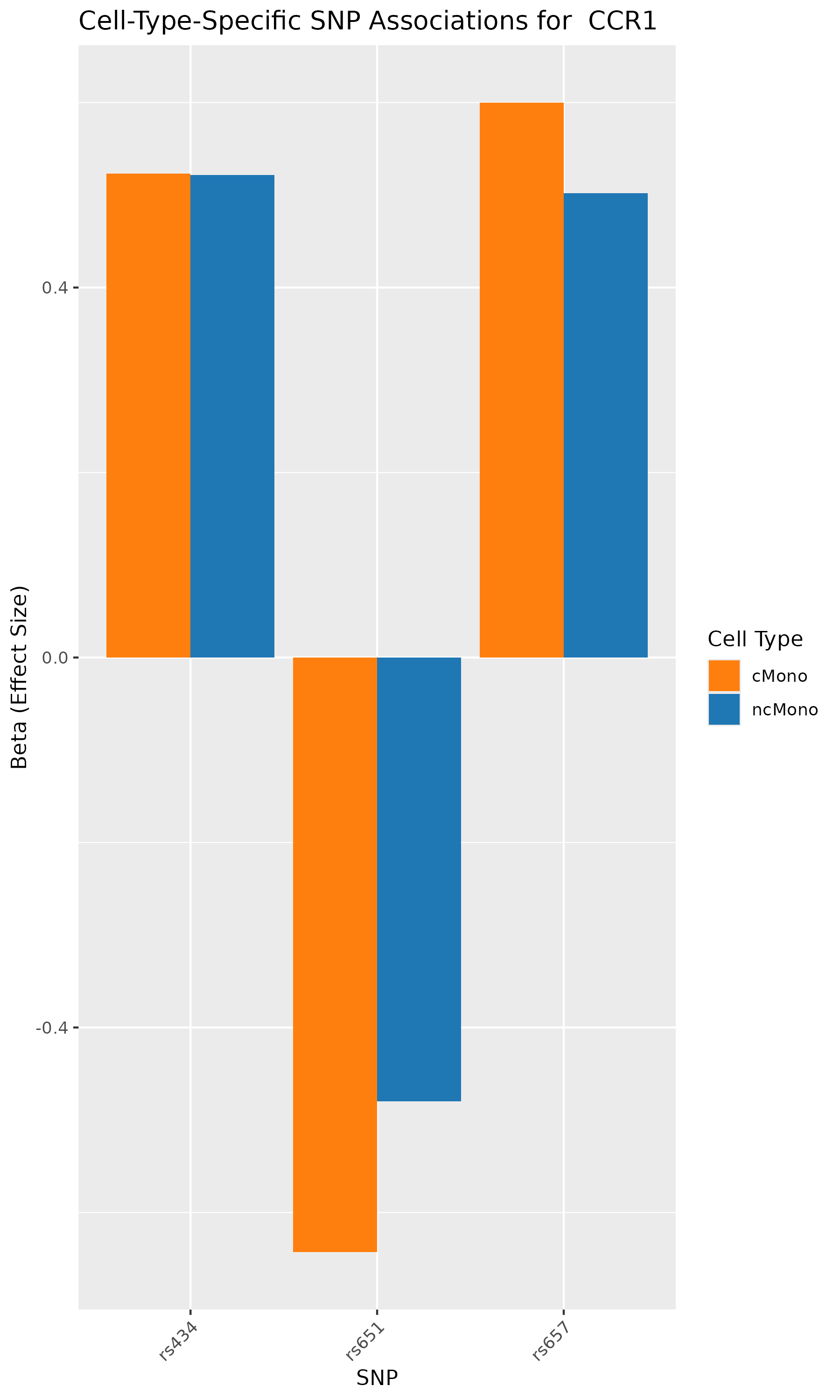
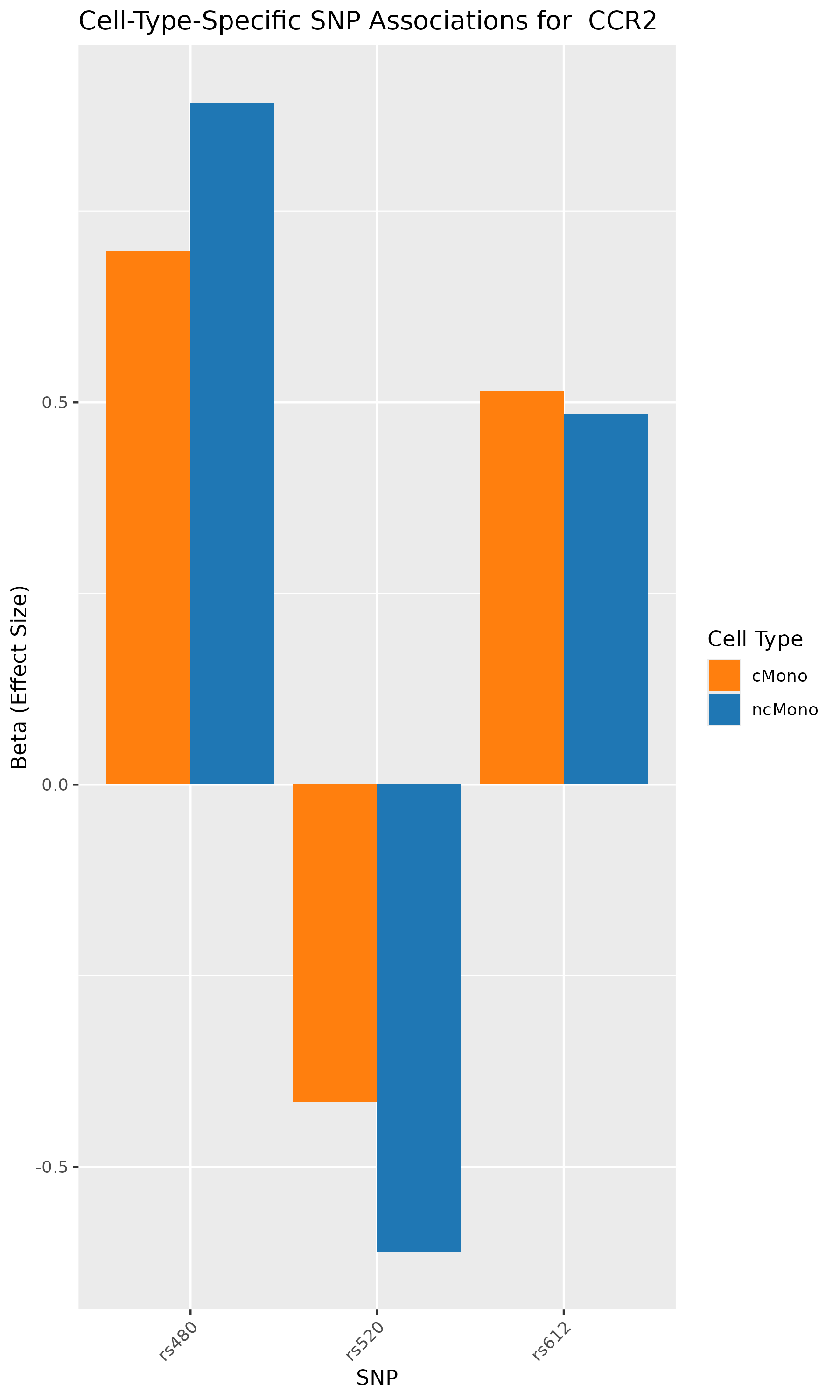
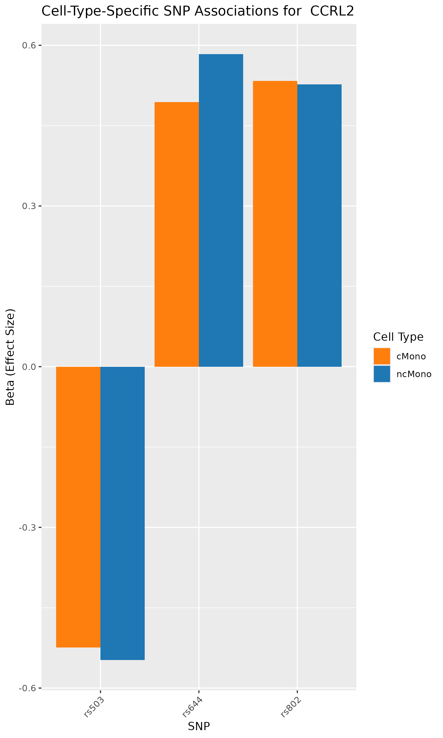
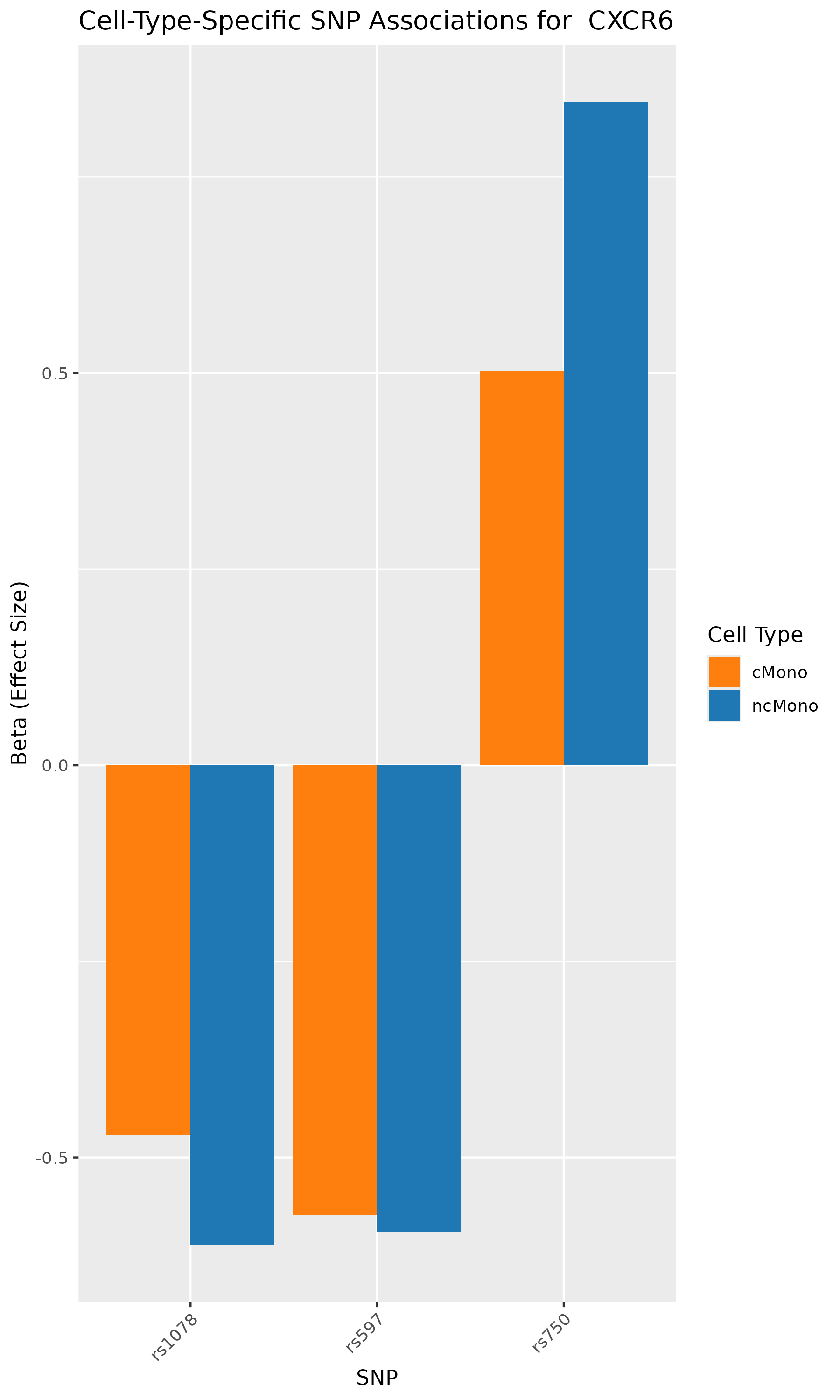
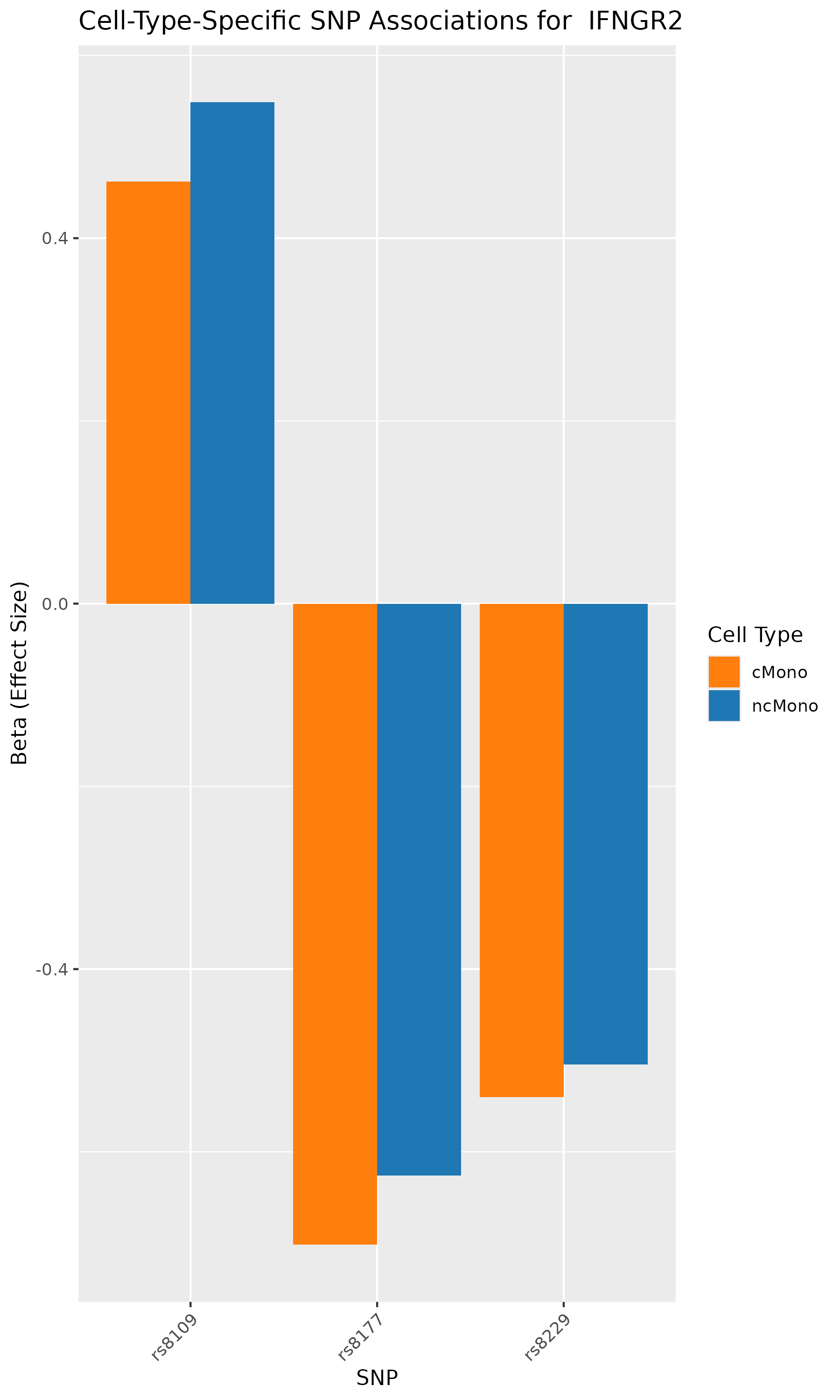
In conclusion, we used the published research study/data, repeated the analyses, and conducted GWAS summary-based SNP-to-chromatin accessibility association analysis to show how genetic variations are associated with chromatin accessibility in a cell-type specific manner. Our results identified the same group of genes and cell types as published in the paper. This analysis presents an approach to approximating a cell-type-resolved chromatin accessibility (caQTL) analysis using public GWAS summary data and chromatin accessibility profiles.
The code used is available caQTL_analysis.